Train a Mask R-CNN model on your own data

Get started with object detection and segmentation.

Computers have always been good at number crunching, but analyzing the huge amount of data in images still brought them to their knees. Until recently that is, when libraries for graphics processing units were created to do more than just play games. We can now harness the raw power of thousands of cores to unlock the meanings behind the pictures.

Using Your Data

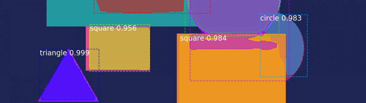
We’re going to be working with an example shape dataset, which has different sizes and colors of circles, squares, and triangles on randomly colored backgrounds. I’ve already went ahead and created a COCO-style version. If you want to learn how to convert your own dataset, take a look at the previous article.

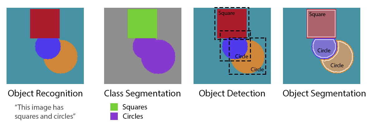
This time our focus will be to automatically label all the shapes in an image and find out where each of them are, down to the pixel. This type of task is called “object segmentation”. During your exploration of computer vision you may have also come across terms like “object recognition”, “class segmentation”, and “object detection”. These all sound similar and can be confusing at first, but seeing what they do helps clear it up. Below are examples of what kind of information we get from each of the four types. Tasks become more difficult as we move from left to right.

Types of image processing

Object recognition tells us what is in the image, but not where or how much. Class segmentation adds position information to the different types of objects in the image. Object detection separates out each object with a rough bounding box. And finally, the hardest of the four, and the one we’ll be training for, object segmentation. It gives every shape a clear boundary, which can also be used to create the results from the previous three.

With a simple dataset like the one we’re using here, we could probably use old school computer vision ideas like Hough (pronounced Huff) circle and line detection or template matching to get pretty good results. But by using deep learning we don’t have to change our approach much to get the same type of results on nearly any type of image dataset. And all without having to think about which exact features we’re looking for. It’s almost magic.

What Is Mask R-CNN?

Before we jump into training our own Mask R-CNN model, let’s quickly break down what the different parts of the name mean. We’ll start from right to left, since that’s the order they were invented.

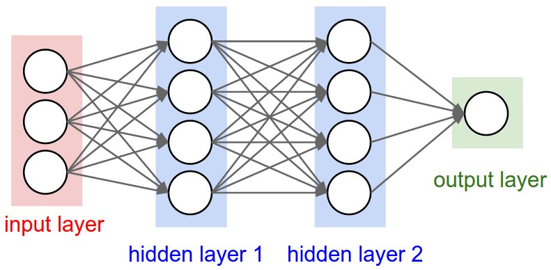
“NN”s are neural networks. They’re an idea inspired by how we imagined biological neurons worked. A neural network is a collection of connected neurons and each neuron outputs a signal depending on its inputs and internal parameters. When we train a neural network, we adjust neuron internal parameters to create the outputs we expect.

Neural Network

The “C” stands for “convolutional”. CNNs were designed specifically for learning with images, but are otherwise similar to standard neural networks. They learn filters that slide (“convolve”) across and down images in small sections at time, instead of going through the entire image at once. CNNs use less parameters and memory than regular neural networks, which allows them to work on much larger images than a traditional neural network.

Convolution

Plain CNNs are good at object recognition, but if we want to do object detection we need to know where things are. That’s where the “R”, for “region” comes in. R-CNNs are able to draw bounding boxes around the objects they find. Over time there have been improvements to the original R-CNN to make them faster, and as you might expect they were called Fast R-CNN and Faster R-CNN. Faster R-CNN adds a Region Proposal Network at the end of a CNN to, you guessed it, propose regions. Those regions are then used as bounding boxes if an object is found inside them.

And finally the “Mask” part of the name is what adds pixel level segmentation and creates our object segmentation model. It adds an additional branch to the network to create binary masks which are similar to the ones we make when annotating images.

Okay, that’s a short overview of what the different parts mean and do. You can find more information on each of them in the References and Resources below. Now let’s get started with actually training our own version of Mask-RCNN.

Get Your Computer Ready

To run the examples you’re going to need an Ubuntu 16.04 system with a recent nvidia graphics card. I was able to train a small part of the network using a GeForce 940M with only 2GB of memory, but you’re better off trying to use an nvidia card with 11GB of memory or more. If you don’t have access one of those you can get started with Amazon Web Services or Google Cloud.

To make sure we’re all on the same page we’ll be using Docker to run everything. Docker uses scripts to create copies of systems, so you don’t have to worry about installing all the little things yourself. But before we can benefit from having things set up automatically for us, first we need to get our host system ready. This part can be a bit of a pain, but it’ll be worth it, I promise.

After installing Ubuntu 16.04, we need to install nvidia graphics drivers and CUDA (a platform for parallel computing). Start by opening a terminal and running the following commands to install the graphics drivers.

sudo add-apt-repository ppa:graphics-drivers/ppa
sudo apt-get update
sudo apt-get install nvidia-graphics-drivers-390

Then continue with installing CUDA.

wget https://developer.nvidia.com/compute/cuda/9.1/Prod/local_installers/cuda-repo-ubuntu1604-9-1-local_9.1.85-1_amd64
sudo dpkg -i cuda-repo-ubuntu1604-9-1-local_9.1.85-1_amd64.deb
sudo apt-key add /var/cuda-repo-<version>/7fa2af80.pub
sudo apt-get update
sudo apt-get install cuda-toolkit-9-1 cuda-libraries-dev-9-1 cuda-libraries-9-1

Now we have to install Docker, Docker-Compose, and Nvidia-Docker.

wget -O get_docker.sh get.docker.com
chmod +x get_docker.sh
sudo ./get_docker.sh
sudo apt-get install -y --allow-downgrades docker-ce=18.03.1~ce-0~ubuntu
sudo usermod -aG docker $USER

sudo curl -L https://github.com/docker/compose/releases/download/1.21.0/docker-compose-$(uname -s)-$(uname -m) -o /usr/local/bin/docker-compose
sudo chmod +x /usr/local/bin/docker-compose

curl -s -L https://nvidia.github.io/nvidia-docker/gpgkey | sudo apt-key add -
distribution=$(. /etc/os-release;echo $ID$VERSION_ID)
curl -s -L https://nvidia.github.io/nvidia-docker/$distribution/nvidia-docker.list | sudo tee /etc/apt/sources.list.d/nvidia-docker.list
sudo apt-get update
sudo apt-get install -y nvidia-docker2
sudo pkill -SIGHUP dockerd

Whew, that was a lot of commands to run. Hopefully everything installed okay and now we can actually start running our Mask R-CNN system. Restart your computer to make sure everything got applied before continuing.

Start Exploring

Download and extract deep-learning-explorer. Inside you’ll find a mask-rcnn folder and a data folder. There’s another zip file in the data/shapes folder that has our test dataset. Extract the shapes.zip file and move annotations, shapes_train2018, shapes_test2018, and shapes_validate2018 to data/shapes.

Back in a terminal, cd into mask-rcnn/docker and run docker-compose up. When you run this command the first time Docker will build the system from scratch, so it may take a few minutes to get ready. Every time after that though it will be ready almost immediately. Once it’s ready you should see something like this:

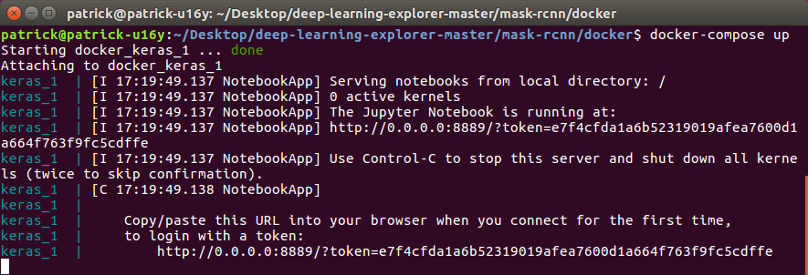Docker system ready

Copy-and-paste that last line into a web browser and you’ll be in Jupyter Notebook. Go to home/keras/mask-rcnn/notebooks and click on mask_rcnn.ipynb. Now you can step through each of the notebook cells and train your own Mask R-CNN model. Behind the scenes Keras with Tensorflow are training neural networks on GPUs. If you don’t have 11GB of graphics card memory, you may run into issues during the “Fine-tuning” step, but you should be able train just the top of the network with cards with as little as 2GB of memory.

The reason we can get fairly good results without having to spend days or weeks training our model, and without having thousands of examples, is because we copied weights (internal neuron parameters) from training done previously on the real COCO dataset. Since most image datasets have similar basic features like colors, and patterns, data from training one model can usually be used for training another. Copying data this way is called Transfer learning.

If you scroll to the bottom of the notebook you’ll notice that we only predict the right shape about 37% of the time. You can help make the model better by increasing the STEPS_PER_EPOCH up to 750 (the total amount of training samples) and running for 5 or more epochs.

During or after training, you can look at some graphs to see how things are going using TensorBoard. We’ll need to log into the Docker container we just started and run TensorBoard before we can access it in our web browser. In a terminal, run docker ps. This will show you all running containers. Use the first two characters of the CONTAINER ID to start a bash shell inside the Docker container training our model. For example, of our ID was d5242f7ab1e3 we would log in using docker exec -it d5 bash. Now that we’re in our container, run tensorboard --logdir ~/data/shapes/logs --host 0.0.0.0 and you should be able to visit http://localhost:8877 to access TensorBoard.

TensorBoard

Now you’re ready to train a Mask R-CNN model on your own data. Let me know what other kinds of models you think would be interesting to explore.

References and Resources

• deep-learning-explorer
• pycococreator – transform your data
• R-CNN (arxiv)
• Fast R-CNN (arxiv)
• Faster R-CNN (arxiv)
• Mask R-CNN (arxiv)
• Stanford CS class notes

Additional Links

• Previous post: Create your own COCO-style datasets